Weight uncertainty in neural networks

Key Idea:

New methods to fulfill old dreams. Long before people modeled weights in neural networks with probabilistic distributions and output posterior mean. But the intractability is always an issue. In this paper author proposes some numerical scheme to approximate.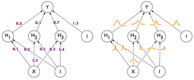

Left: Traditional deterministic neural networks. Right: Bayesian neural networks. From [1]

Lemma:
Let $\epsilon $ be a random variable having a probability density given by $q(\epsilon)$ and let $w=t(\theta, \epsilon)$ where $t(\theta, \epsilon)$ is a deterministic function. Suppose further that the marginal probability density of $w, q(w | \theta)$, is such that $q(\epsilon) d\epsilon = q(w|\theta) dw$ . Then for function $f$ with derivatives in $w$:
$\frac{\partial}{\partial \theta} \mathbb{E}_{q(\mathbf{w} | \theta)}[f(\mathbf{w}, \theta)]=\mathbb{E}_{q(\epsilon)}\left[\frac{\partial f(\mathbf{w}, \theta)}{\partial \mathbf{w}} \frac{\partial \mathbf{w}}{\partial \theta}+\frac{\partial f(\mathbf{w}, \theta)}{\partial \theta}\right]$

Proof: 
$$
\begin{aligned} \frac{\partial}{\partial \theta} \mathbb{E}_{q(\mathbf{w} | \theta)}[f(\mathbf{w}, \theta)] &=\frac{\partial}{\partial \theta} \int f(\mathbf{w}, \theta) q(\mathbf{w} | \theta) \mathrm{d} \mathbf{w} \\ &=\frac{\partial}{\partial \theta} \int f(\mathbf{w}, \theta) q(\epsilon) \mathrm{d} \epsilon \\ &=\mathbb{E}_{q(\epsilon)}\left[\frac{\partial f(\mathbf{w}, \theta)}{\partial \mathbf{w}} \frac{\partial \mathbf{w}}{\partial \theta}+\frac{\partial f(\mathbf{w}, \theta)}{\partial \theta}\right] \end{aligned}
$$

Variational approximation to Bayesian posterior distribution on the weights:
$$
\begin{aligned} \theta^{\star} &=\arg \min _{\theta} \mathrm{KL}[q(\mathbf{w} | \theta) \| P(\mathbf{w} | \mathcal{D})] \\

 &=\arg \min _{\theta} \int q(\mathbf{w} | \theta) \log \frac{q(\mathbf{w} | \theta)}{P(\mathbf{w}) P(\mathcal{D} | \mathbf{w})} \mathrm{d} \mathbf{w} \\

&=\arg \min _{\theta} \mathrm{KL}[q(\mathbf{w} | \theta) \| P(\mathbf{w})]-\mathbb{E}_{q(\mathbf{w} | \theta)}[\log P(\mathcal{D} | \mathbf{w})]
 \end{aligned}
$$
The resulting cost function is called variational free energy or expected lower-bound
$\mathcal{F}(\mathcal{D}, \theta)=\mathrm{KL}[q(\mathbf{w} | \theta) \| P(\mathbf{w})]
- \mathbb{E}_{q(\mathbf{w} | \theta)}[\log P(\mathcal{D} | \mathbf{w})]$

We approximate it:
$\mathcal{F}(\mathcal{D}, \theta) \approx \sum_{i=1}^{n} \log q\left(\mathbf{w}^{(i)} | \theta\right)-\log P\left(\mathbf{w}^{(i)}\right) - \log P\left(\mathcal{D} | \mathbf{w}^{(i)}\right)$

where $w^{(i)}$ denotes  the ith Monte Carlo sample drawn form the variational posterior $q\left(\mathbf{w}^{(i)} | \theta\right)$

Notice that every term of the approximate cost depends on the particular weights drawn from the variational posterior: this is an instance of a variance reduction technique known as common random numbers. The author claims that a prior without an easy-to-compute closed form complexity cost performed best.

Gaussian variational posterior:
Suppose the variational posterior is a diagonal Gaussian distribution, then a sample of the weights $w$ can be obtained by sampling a unit Gaussian, shifting it by mean $\mu$ and scaling by a standard deviation $\sigma$.

$\sigma=\log(1+ exp(\rho))$
$\theta=(\mu, \rho)$
$\mathbf{w}=t(\theta, \epsilon)=\mu+\log (1+\exp (\rho)) \circ \epsilon$

class Gaussian(object):
    def __init__(self, mu, rho):
        super().__init__()
        self.mu = mu
        self.rho = rho
        self.normal = torch.distributions.Normal(0,1)
    
    @property
    def sigma(self):
        return torch.log1p(torch.exp(self.rho))
    
    def sample(self):
        epsilon = self.normal.sample(self.rho.size())
        return self.mu + self.sigma * epsilon
    
    def log_prob(self, input):
        return (-math.log(math.sqrt(2 * math.pi))
                - torch.log(self.sigma)
                - ((input - self.mu) ** 2) / (2 * self.sigma ** 2)).sum()

Note:

torch.log1p(input, output=None) 

is more accurate than

torch.log() 

for small values of input 

Optimisation steps:

1. Sample $\epsilon \sim \mathcal{N}(0, I)$
2. Let $\mathbf{w}=\mu+\log (1+\exp (\rho)) \circ \epsilon$
3. Let $\theta=(\mu, \rho)$
4. Let $f(\mathbf{w}, \theta)=\log q(\mathbf{w} | \theta)-\log P(\mathbf{w}) P(\mathcal{D} | \mathbf{w})$
5. Gradient w.r.t the mean:$\Delta_{\mu}=\frac{\partial f(\mathbf{w}, \theta)}{\partial \mathbf{w}}+\frac{\partial f(\mathbf{w}, \theta)}{\partial \mu}$
6. Calculate the gradient w.r.t. the standard deviation parameter $\rho$: $\Delta_{\rho}=\frac{\partial f(\mathbf{w}, \theta)}{\partial \mathbf{w}} \frac{\epsilon}{1+\exp (-\rho)}+\frac{\partial f(\mathbf{w}, \theta)}{\partial \rho}$
7. Update the variational parameters: 

\begin{array}{c}{\mu \leftarrow \mu-\alpha \Delta_{\mu}} \\ {\rho \leftarrow \rho-\alpha \Delta_{\rho}}\end{array}

Scale mixture prior

The author propose a scale mixture of two Gaussians densities as the prior. Each density is zero-mean-ed, but having differing variances.
$$
P(\mathbf{w})=\prod_{j} \pi \mathcal{N}\left(\mathbf{w}_{j} | 0, \sigma_{1}^{2}\right)+(1-\pi) \mathcal{N}\left(\mathbf{w}_{j} | 0, \sigma_{2}^{2}\right)
$$

$$
\log P(\mathbf{w})=\sum_{j} \log \left(\pi \mathcal{N}\left(\mathbf{w}_{j} | 0, \sigma_{1}^{2}\right)+(1-\pi) \mathcal{N}\left(\mathbf{w}_{j} | 0, \sigma_{2}^{2}\right)\right)
$$

where $w_j$ is the $j$th weight of the network. $\sigma_1^2$ and $\sigma_2^2$ are the variances of the mixture components. The first mixture component of the prior is giving a larger variance than the second, i.e., $\sigma_1 \gt \sigma_2$, providing a heavier tail in the prior density that a plain Gaussian prior.  The second mixture component has a small variance $\sigma_2 \ll 1$ causing many of the weights to a priori tightly concentrate around zero.

 
class ScaleMixtureGaussian(object):
    def __init__(self, pi, sigma1, sigma2):
        super().__init__()
        self.pi = pi
        self.sigma1 = sigma1
        self.sigma2 = sigma2
        self.gaussian1 = torch.distributions.Normal(0,sigma1)
        self.gaussian2 = torch.distributions.Normal(0,sigma2)
    
    def log_prob(self, input):
        prob1 = torch.exp(self.gaussian1.log_prob(input))
        prob2 = torch.exp(self.gaussian2.log_prob(input))
        return (torch.log(self.pi * prob1 + (1-self.pi) * prob2)).sum()

Minibatches and KL re-weighting:

If minibatches are partitioned uniformly at random, the KL cost can be distributed non-uniformly among the minibatches at each epoch. Let $\pi \in [0, 1]^M$ and $\sum_{i=1}^M \pi_i =1 $, and define:

$$
\begin{array}{r}{\mathcal{F}_{i}^{\pi}\left(\mathcal{D}_{i}, \theta\right)=\pi_{i} \mathrm{KL}[q(\mathbf{w} | \theta) \| P(\mathbf{w})]} \\ {-\mathbb{E}_{q(\mathbf{w} | \theta)}\left[\log P\left(\mathcal{D}_{i} | \mathbf{w}\right)\right]}\end{array}
$$

Then $\mathbb{E}_{M}\left[\sum_{i=1}^{M} \mathcal{F}_{i}^{\pi}\left(\mathcal{D}_{i}, \theta\right)\right]=\mathcal{F}(\mathcal{D}, \theta)$ where $E_M$ denotes an expectation over the random partitioning of minibatches.  The author suggests that $\pi_i= \frac{2^{M-i}}{ 2^M -1}$ works well.

Ref:

1. Wikipedia Contributors. (2019, March 11). Variance reduction. Retrieved August 8, 2019,  https://en.wikipedia.org/wiki/Variance_reduction
2. Nitarshan Rajkumar. (2018). Weight Uncertainty in Neural Networks. Retrieved August 13, 2019, https://www.nitarshan.com/bayes-by-backprop

‌