LSTM (2)

Long Short-Term Memory (LSTM)

On step t, there is a hidden state $h^{(t)}$ and a cell state $c^{(t)}$:

• Both are vectors of length n 
• The cell stores long-term information 
• The LSTM can erase, write or read information from the cell 

Formulas(Note, all $\sigma $ represent sigmoid function)

Forget gate: controls what is kept vs forgotten, from previous cell state

$\boldsymbol{f}^{(t)}=\sigma \left(\boldsymbol{W}_{f} \boldsymbol{h}^{(t-1)}+\boldsymbol{U}_{f} \boldsymbol{x}^{(t)}+\boldsymbol{b}_{f}\right)$

Input gate: controls what parts of the new cell content are written to cell

$\boldsymbol{i}^{(t)}=\sigma \left(\boldsymbol{W}_{i} \boldsymbol{h}^{(t-1)}+\boldsymbol{U}_{i} \boldsymbol{x}^{(t)}+\boldsymbol{b}_{i}\right)$

Output gate: controls what parts of cell are output to hidden state

$\boldsymbol{o}^{(t)}=\sigma \left(\boldsymbol{W}_{o} \boldsymbol{h}^{(t-1)}+\boldsymbol{U}_{o} \boldsymbol{x}^{(t)}+\boldsymbol{b}_{o}\right)$

New cell content: this is the new content to be written to the cell

$\tilde{\boldsymbol{c}}^{(t)}=\tanh \left(\boldsymbol{W}_{c} \boldsymbol{h}^{(t-1)}+\boldsymbol{U}_{c} \boldsymbol{x}^{(t)}+\boldsymbol{b}_{c}\right)$

Cell state: erase (“forget”) some content from last cell state, and write (“input”) some new cell content

$\boldsymbol{c}^{(t)}=\boldsymbol{f}^{(t)} \circ \boldsymbol{c}^{(t-1)}+\boldsymbol{i}^{(t)} \circ \tilde{\boldsymbol{c}}^{(t)}$

Hidden state: read (“output”) some content from the cell

$\boldsymbol{h}^{(t)}=\boldsymbol{o}^{(t)} \circ \tanh \boldsymbol{c}^{(t)}$

LSTM Diagram. Source: 苏剑林

Ref: 

1. CS224n: Natural Language Processing with Deep Learning, Lecture 7
2. 苏剑林, ON-LSTM：用有序神经元表达层次结构

Fusion of Detected Objects in Text for Visual Question Answering

Models:

B2T2: Bounding Boxes in Text Transformer 

Concepts:

Late fusion: Text and image that are integrated late
Early fusion: The processing of one be conditioned on the analysis of the other 

Data:= $(I , B, T, I)$

• $I$ is an image
• $B=[b_1, b_2, ..., b_m ]$ a list of bounding boxes referring to regions of $I$, where each $b_i $ is identified by the lower left corner, height and width
• $T=[t_1, ..., t_n]$ is a passage of tokenized text (some tokens are not natural language but references to $B$)
• $l$ is a numeric class label in $\{ 0, 1\}$

B2T2:=

model the class distribution as:

$$p(l | T, I , B, R)= \frac{e^{\phi (E'(T, I, B, R))*a_l + b_l}}
{\sum_{l'}  e^{\phi (E'(T, I, B, R))*a_{l'} + b_{l'}} }
$$

$$
E'(T, I, B, R)= E(T) + \sum_{i=1}^m R_i [M \Phi(crop(I, b_i)) + \pi (b_i)]^T
$$

where $M$ is a learnt matrix, $\Phi$ can be a resnet, $\pi(b_i)$ denotes the embedding of $b_i$'s shape and position information in $R^d$

Gradient Boosting Trees

What is gradient boosting

A kind of boosting using functional gradient descent. It uses weak learner to fit gradient residuals and then add to original learner, thus making an ensemble. 

Source: Wikipedia

XGBOOST

$$\text{obj}(\theta) = L(\theta) + \Omega(\theta)$$

where $L$ is the training loss function, and $Ω$ is the regularization term. The training loss measures how predictive our model is with respect to the training data. A common choice of L is the mean squared error, which is given by
$$
L(\theta) = \sum_i (y_i-\hat{y}_i)^2
$$

$$
\text{obj} = \sum_{i=1}^n l(y_i, \hat{y}_i^{(t)}) + \sum_{i=1}^t\Omega(f_i)
$$


Additive Training:
$$
\begin{split}\hat{y}_i^{(0)} &= 0\\
\hat{y}_i^{(1)} &= f_1(x_i) = \hat{y}_i^{(0)} + f_1(x_i)\\
\hat{y}_i^{(2)} &= f_1(x_i) + f_2(x_i)= \hat{y}_i^{(1)} + f_2(x_i)\\
&\dots\\
\hat{y}_i^{(t)} &= \sum_{k=1}^t f_k(x_i)= \hat{y}_i^{(t-1)} + f_t(x_i)\end{split}
$$

For step t:
$$
\begin{split}\text{obj}^{(t)} & = \sum_{i=1}^n l(y_i, \hat{y}_i^{(t)}) + \sum_{i=1}^t\Omega(f_i) \\
          & = \sum_{i=1}^n l(y_i, \hat{y}_i^{(t-1)} + f_t(x_i)) + \Omega(f_t) + \mathrm{constant}\end{split}
$$

For L2 loss:
$$
\begin{split}\text{obj}^{(t)} & = \sum_{i=1}^n (y_i - (\hat{y}_i^{(t-1)} + f_t(x_i)))^2 + \sum_{i=1}^t\Omega(f_i) \\
          & = \sum_{i=1}^n [2(\hat{y}_i^{(t-1)} - y_i)f_t(x_i) + f_t(x_i)^2] + \Omega(f_t) + \mathrm{constant}\end{split}
$$

$$
\text{obj}^{(t)} = \sum_{i=1}^n [l(y_i, \hat{y}_i^{(t-1)}) + g_i f_t(x_i) + \frac{1}{2} h_i f_t^2(x_i)] + \Omega(f_t) + \mathrm{constant}
$$

where
$$
\begin{split}g_i &= \partial_{\hat{y}_i^{(t-1)}} l(y_i, \hat{y}_i^{(t-1)})\\
h_i &= \partial_{\hat{y}_i^{(t-1)}}^2 l(y_i, \hat{y}_i^{(t-1)})\end{split}
$$

So:
$$
\textrm{obt}^{(t)}=\sum_{i=1}^n [g_i f_t(x_i) + \frac{1}{2} h_i f_t^2(x_i)] + \Omega(f_t)
$$

Regularization 



Redefine each tree as:
$$
f_t(x) = w_{q(x)}, w \in R^T, q:R^d\rightarrow \{1,2,\cdots,T\}
$$

Here w is the vector of scores on leaves, q is a function assigning each data point to the corresponding leaf, and T is the number of leaves. In XGBoost, we define the complexity as

$$
\Omega(f) = \gamma T + \frac{1}{2}\lambda \sum_{j=1}^T w_j^2
$$

Reformatting:

$$
\begin{split}\text{obj}^{(t)} &\approx \sum_{i=1}^n [g_i w_{q(x_i)} + \frac{1}{2} h_i w_{q(x_i)}^2] + \gamma T + \frac{1}{2}\lambda \sum_{j=1}^T w_j^2\\
&= \sum^T_{j=1} [(\sum_{i\in I_j} g_i) w_j + \frac{1}{2} (\sum_{i\in I_j} h_i + \lambda) w_j^2 ] + \gamma T\end{split}
$$

where Ij={i|q(xi)=j} is the set of indices of data points assigned to the j-th leaf. Notice that in the second line we have changed the index of the summation because all the data points on the same leaf get the same score. We could further compress the expression by defining:

$G_j = \sum_{i\in I_j} g_i$

$H_j = \sum_{i\in I_j} h_i$

$$
\text{obj}^{(t)} = \sum^T_{j=1} [G_jw_j + \frac{1}{2} (H_j+\lambda) w_j^2] +\gamma T
$$


The theoretical best solution is:
$$
\begin{split}w_j^\ast &= -\frac{G_j}{H_j+\lambda}\\
\text{obj}^\ast &= -\frac{1}{2} \sum_{j=1}^T \frac{G_j^2}{H_j+\lambda} + \gamma T\end{split}
$$


Splitting criterion:
$$
Gain = \frac{1}{2} \left[\frac{G_L^2}{H_L+\lambda}+\frac{G_R^2}{H_R+\lambda}-\frac{(G_L+G_R)^2}{H_L+H_R+\lambda}\right] - \gamma
$$

Ref:

1. https://xgboost.readthedocs.io/en/latest/tutorials/model.html
2. https://github.com/MSusik/newgradientboosting/blob/master/pydata.pdf

Attention Mechanism

Why attention? 

Resource saving

• Only need sensors where relevant bits are
(e.g. fovea vs. peripheral vision)
• Only compute relevant bits of information
(e.g. fovea has many more ‘pixels’ than periphery)

Variable state manipulation

• Manipulate environment (for all grains do: eat)
• Learn modular subroutines (not state)

Some forms of attention that you might not notice:

• Watson Nadaraya Estimator
•  Pooling
• Iterative Pooling 
• 
  

Ref:

1. Alex Smola and Aston Zhang, Attention in Deep Learning, ICML 2019 Tutorial , Slides link 
2. 
   

Mutual Information

Mutual Information 
$$
I(X ; Y)=D_{\mathrm{KL}}\left(P_{(X, Y)} \| P_{X} \otimes P_{Y}\right)

$$


Intuitively, mutual information measures the information that $X$ and $Y$ share: It measures how much knowing one of these variables reduces uncertainty about the other.

\begin{aligned} \mathrm{I}(X ; Y) & \equiv \mathrm{H}(X)-\mathrm{H}(X | Y) \\ & \equiv \mathrm{H}(Y)-\mathrm{H}(Y | X) \\ & \equiv \mathrm{H}(X)+\mathrm{H}(Y)-\mathrm{H}(X, Y) \\ & \equiv \mathrm{H}(X, Y)-\mathrm{H}(X | Y)-\mathrm{H}(Y | X) \end{aligned}

where $H(Y|X)$ means Conditional Entropy, defined as:


$$

\mathrm{H}(Y | X)=-\sum_{x \in \mathcal{X}, y \in \mathcal{Y}} p(x, y) \log \frac{p(x, y)}{p(x)}

$$

$$
\begin{aligned} \mathrm{H}(Y | X) & \equiv \sum_{x \in \mathcal{X}} p(x) \mathrm{H}(Y | X=x) \\ &=-\sum_{x \in \mathcal{X}} p(x) \sum_{y \in \mathcal{Y}} p(y | x) \log p(y | x) \\ &=-\sum_{x \in \mathcal{X}} \sum_{y \in \mathcal{Y}} p(x, y) \log p(y | x) \\ &=-\sum_{x \in \mathcal{X}, y \in \mathcal{Y}} p(x, y) \log p(y | x) \\ &=-\sum_{x \in \mathcal{X}, y \in \mathcal{Y}} p(x, y) \log \frac{p(x, y)}{p(x)} \\ &=\sum_{x \in \mathcal{X}, y \in \mathcal{Y}} p(x, y) \log \frac{p(x)}{p(x, y)} \end{aligned}

$$

RNN and LSTM

RNN

Assume the RNN is with the following architecture, with hyperbolic tangent activation function, output is discrete.

From time $t=1$ to $t=\tau$ , we apply the update equations:

$\begin{aligned} \boldsymbol{a}^{(t)} &=\boldsymbol{b}+\boldsymbol{W} \boldsymbol{h}^{(t-1)}+\boldsymbol{U} \boldsymbol{x}^{(t)} \\ \boldsymbol{h}^{(t)} &=\tanh \left(\boldsymbol{a}^{(t)}\right) \\ \boldsymbol{o}^{(t)} &=\boldsymbol{c}+\boldsymbol{V} \boldsymbol{h}^{(t)} \\ \hat{\boldsymbol{y}}^{(t)} &=\operatorname{softmax}\left(\boldsymbol{o}^{(t)}\right) \end{aligned}$

The total loss for a given sequence of $x$ values paired with a sequence of $y$ values would then be just the sum of the losses over all the time steps. If $L^{(t)}$  is the negative log-likelihood of $y^{(t)}$ given $x^{(1)}, x^{(2)}, ..., x^{(t)}$, then

$\begin{aligned} & L\left(\left\{\boldsymbol{x}^{(1)}, \ldots, \boldsymbol{x}^{(\tau)}\right\},\left\{\boldsymbol{y}^{(1)}, \ldots, \boldsymbol{y}^{(\tau)}\right\}\right) \\=& \sum_{t} L^{(t)} \\=&-\sum_{t} \log p_{\text {model }}\left(y^{(t)} |\left\{\boldsymbol{x}^{(1)}, \ldots, \boldsymbol{x}^{(t)}\right\}\right) \end{aligned}$

Before deriving the derivative for a RNN, let's see what is the derivative for a softmax function.

Denote:
$D_{j} S_{i}=\frac{\partial S_{i}}{\partial a_{j}}=\frac{\partial \frac{e^{a_{i}}}{\sum_{k=1}^{N} e^{a_{k}}}}{\partial a_{j}}$

$D_{j} S_{i}=\left\{\begin{array}{cc}{S_{i}\left(1-S_{j}\right)} & {i=j} \\ {-S_{j} S_{i}} & {i \neq j}\end{array}\right.$

Namely:

$D_{j} S_{i}=S_{i}\left(\delta_{i j}-S_{j}\right)$

Gradient in RNN

For each node $\boldsymbol{N}$:

$$\frac{\partial L}{\partial L^{(t)}}=1$$


\begin{equation}
\begin{split}

\left(\nabla_{o^{(t)}} L\right)_{i} & =\frac{\partial L}{\partial o_{i}^{(t)}} \\

 & =\frac{\partial L}{\partial L^{(t)}} \frac{\partial L^{(t)}}{\partial o_{j}^{(t)}}  \\

 &= 1 \times \frac{\partial (- log \hat{y}^{(t)}_{y^{(t)}})} {\partial \hat{y}^{(t)}_{y^{(t)}}} 

\frac{\partial \hat{y}^{(t)}_{y^{(t)}}} {\partial o_{i}^{(t)}} \\

& = \hat{y}_{i}^{(t)}-\mathbf{1}_{i,y^{(t)}}

\end{split}
\end{equation}

LSTM

LSTM architecture from Deep Learning book

Forget gate:   $$ f_{i}^{(t)}=\sigma\left(b_{i}^{f}+\sum_{j} U_{i, j}^{f} x_{j}^{(t)}+\sum_{j} W_{i, j}^{f} h_{j}^{(t-1)}\right) $$

where $\sigma$ is the sigmoid function

Input gate: 
$$
g_{i}^{(t)}=\sigma\left(b_{i}^{g}+\sum_{j} U_{i, j}^{g} x_{j}^{(t)}+\sum_{j} W_{i, j}^{g} h_{j}^{(t-1)}\right)

$$

Output gate:
$$
q_{i}^{(t)}=\sigma\left(b_{i}^{o}+\sum_{j} U_{i, j}^{o} x_{j}^{(t)}+\sum_{j} W_{i, j}^{o} h_{j}^{(t-1)}\right)

$$

LSTM Cell Internal State:
$$
s_{i}^{(t)}=f_{i}^{(t)} s_{i}^{(t-1)}+g_{i}^{(t)} \sigma\left(b_{i}+\sum_{j} U_{i, j} x_{j}^{(t)}+\sum_{j} W_{i, j} h_{j}^{(t-1)}\right)

$$

Output(hidden state):
$$
h_{i}^{(t)}=\tanh \left(s_{i}^{(t)}\right) q_{i}^{(t)}
$$

Ref:

1. Goodfellow, I., Bengio, Y., & Courville, A. (2016). Deep learning. MIT press.
2. https://eli.thegreenplace.net/2016/the-softmax-function-and-its-derivative/

Neural Networks that can reason?

Categorical reparameterization with Gumbel softmax

Gumbel Distribution

The Gumbel distribution (Generalized Extreme Value distribution Type-I) is used to model the distribution of the maximum (or the minimum) of a number of samples of various distributions.

The CDF is $F(x ; \mu, \beta)=e^{-e^{-(x-\mu) / \beta}}$
the PDF is
 $$
\begin{array}{l}{\frac{1}{\beta} e^{-\left(z+e^{-z}\right)}} \\ {\text { where } z=\frac{x-\mu}{\beta}}\end{array}
$$

The Standard Gumbel Distribution is the case when $\mu=0$ and $\beta=1$
In this case, the CDF is $F(x)= e^{-e^{(-x)}}$
the PDF is $f(x)=e^{-(x+e^{-x})}$

Since the quantile function(inverse cumulative distribution function), $Q(p)$, of a Gumbel distribution is given by
$$Q(p)=\mu-\beta \ln (-\ln (p))$$
the variate  $Q(U)$ has a Gumbel distribution with parameters $\mu$  and $\beta$, when the random variate $U \sim Uniform(0,1)$


The Gumbel Softmax Distribution 

Let $z$ be a categorical variable with class probabilities $\pi_1, \pi_2, ..., \pi_k$. And we assume categorical samples are encoded as k-dimensional one-hot vectors lying on the corners of the (k-1)-dimensional simplex, $\Delta^{k-1}$.
$\mathbb{E}_{p}[z]=\left[\pi_{1}, \ldots, \pi_{k}\right]$

The Gumbel-Max trick provides a simple and efficient way of drawing samples $z$ from a categorical distribution with class probabilities $\pi$.
$$
z=\textrm{one_hot}(\arg \max_i [g_i + \log{\pi_i}])
$$
where $g_1, ..., g_k $ are i.i.d samples drawn from Gumbel(0,1). Then we use softmax as a continuous differentiation approximation to $\arg\max$.

$y\in \Delta^{k-1}$ where

$$y_{i}=\frac{\exp \left(\left(\log \left(\pi_{i}\right)+g_{i}\right) / \tau\right)}{\sum_{j=1}^{k} \exp \left(\left(\log \left(\pi_{j}\right)+g_{j}\right) / \tau\right)} \quad$$ for $i=1, \ldots, k$

$\tau$ is the softmax temperature, and the Gumbel-softmax distribution density is (for derivation, see[1]):

$$p_{\pi, \tau}\left(y_{1}, \ldots, y_{k}\right)=\Gamma(k) \tau^{k-1}\left(\sum_{i=1}^{k} \pi_{i} / y_{i}^{\tau}\right)^{-k} \prod_{i=1}^{k}\left(\pi_{i} / y_{i}^{\tau+1}\right)$$

The Gumbel-Softmax distribution interpolates between discrete one-hot-encoded categorical distributions and continuous categorical densities. 

(a) For low temperatures($\tau=0.1, 0.5$)

the expected value of a Gumbel-Softmax random variable approaches the expected value of a categorical random variable with the same logits. As the temperature increases($\tau=1, 10$), the

expected value converges to a uniform distribution over the categories. (b) Samples from Gumbel Softmax distributions are identical to samples from a categorical distribution as$\tau \to 0$. At higher

temperatures, Gumbel-Softmax samples are no longer one-hot, and become uniform as $\tau \to \infty$

Gumbel-Softmax Estimator

The procedure of replacing non-differentiable categorical samples with a differentiable apprxoimatin during training as the Gumbel-Softmax estimator. Notice there is a trade-off between small temperatures where samples are close to one-hot but gradients have large variances, and large temperatures where samples are smooth(uniform-like) but variance of gradients are small.

The author suggests a annealing scheme(entropy regularization) to learn this parameter $\tau$

For scenarios in which we are constrained to sampling discrete values, we discretize $y$ using argmax but use continuous approximation in the backward pass by let $\nabla_\theta z \approx \nabla_\theta y$. This is the Straight-Through(ST) Gumbel Estimator

Related Methods:

See the picture.
(a): If $x(\theta)$ is deterministic and differentiable, $\nabla_\theta f(x)$ can be computed via backprop directly
(b):





Ref:

1. Jang, E., Brain, G., Gu, S., & Poole, B. (n.d.). Published as a conference paper at ICLR 2017 CATEGORICAL REPARAMETERIZATION WITH GUMBEL-SOFTMAX. 
2. Wikipedia Contributors. (2019, August 12). Gumbel distribution. Wikipedia. Wikimedia Foundation. https://en.wikipedia.org/wiki/Gumbel_distribution. 
3. 
   

Different perspectives on importance weight autoencoders

The importance-weighted autoencoder (IWAE) approach of Burda et al.[1] defines a sequence of increasingly tighter bounds on the marginal likelihood of latent variable models. Recently, Cremer et al.[2] reinterpreted the IWAE bounds as ordinary variational evidence lower bounds (ELBO) applied to increasingly accurate variational distributions. In this work, we provide yet another perspective on the IWAE bounds. We interpret each IWAE bound as a biased estimator of the true marginal likelihood where for the bound defined on K samples we show the bias to be of order O(1/K). In our theoretical analysis of the IWAE objective we derive asymptotic bias and variance expressions. Based on this analysis we develop jackknife variational inference (JVI), a family of bias-reduced estimators reducing the bias to O(K^{-(m+1)}) for any given m < K while retaining computational efficiency. Finally, we demonstrate that JVI leads to improved evidence estimates in variational autoencoders. We also report first results on applying JVI to learning variational autoencoders.

Microsoft Research

Ref:

1. Burda, Y., Grosse, R., & Salakhutdinov, R. (2016). IMPORTANCE WEIGHTED AUTOENCODERS. 
2. Cremer, C., Morris, Q., & Duvenaud, D. (n.d.). Workshop track -ICLR 2017 REINTERPRETING IMPORTANCE-WEIGHTED AUTOENCODERS. 
3. Debiasing Evidence Approximations: On Importance-Weighted Autoencoders and Jackknife Variational Inference

Weight uncertainty in neural networks

Key Idea:

New methods to fulfill old dreams. Long before people modeled weights in neural networks with probabilistic distributions and output posterior mean. But the intractability is always an issue. In this paper author proposes some numerical scheme to approximate.

Left: Traditional deterministic neural networks. Right: Bayesian neural networks. From [1]

Lemma:
Let $\epsilon $ be a random variable having a probability density given by $q(\epsilon)$ and let $w=t(\theta, \epsilon)$ where $t(\theta, \epsilon)$ is a deterministic function. Suppose further that the marginal probability density of $w, q(w | \theta)$, is such that $q(\epsilon) d\epsilon = q(w|\theta) dw$ . Then for function $f$ with derivatives in $w$:
$\frac{\partial}{\partial \theta} \mathbb{E}_{q(\mathbf{w} | \theta)}[f(\mathbf{w}, \theta)]=\mathbb{E}_{q(\epsilon)}\left[\frac{\partial f(\mathbf{w}, \theta)}{\partial \mathbf{w}} \frac{\partial \mathbf{w}}{\partial \theta}+\frac{\partial f(\mathbf{w}, \theta)}{\partial \theta}\right]$

Proof: 
$$
\begin{aligned} \frac{\partial}{\partial \theta} \mathbb{E}_{q(\mathbf{w} | \theta)}[f(\mathbf{w}, \theta)] &=\frac{\partial}{\partial \theta} \int f(\mathbf{w}, \theta) q(\mathbf{w} | \theta) \mathrm{d} \mathbf{w} \\ &=\frac{\partial}{\partial \theta} \int f(\mathbf{w}, \theta) q(\epsilon) \mathrm{d} \epsilon \\ &=\mathbb{E}_{q(\epsilon)}\left[\frac{\partial f(\mathbf{w}, \theta)}{\partial \mathbf{w}} \frac{\partial \mathbf{w}}{\partial \theta}+\frac{\partial f(\mathbf{w}, \theta)}{\partial \theta}\right] \end{aligned}
$$

Variational approximation to Bayesian posterior distribution on the weights:
$$
\begin{aligned} \theta^{\star} &=\arg \min _{\theta} \mathrm{KL}[q(\mathbf{w} | \theta) \| P(\mathbf{w} | \mathcal{D})] \\

 &=\arg \min _{\theta} \int q(\mathbf{w} | \theta) \log \frac{q(\mathbf{w} | \theta)}{P(\mathbf{w}) P(\mathcal{D} | \mathbf{w})} \mathrm{d} \mathbf{w} \\

&=\arg \min _{\theta} \mathrm{KL}[q(\mathbf{w} | \theta) \| P(\mathbf{w})]-\mathbb{E}_{q(\mathbf{w} | \theta)}[\log P(\mathcal{D} | \mathbf{w})]
 \end{aligned}
$$
The resulting cost function is called variational free energy or expected lower-bound
$\mathcal{F}(\mathcal{D}, \theta)=\mathrm{KL}[q(\mathbf{w} | \theta) \| P(\mathbf{w})]
- \mathbb{E}_{q(\mathbf{w} | \theta)}[\log P(\mathcal{D} | \mathbf{w})]$

We approximate it:
$\mathcal{F}(\mathcal{D}, \theta) \approx \sum_{i=1}^{n} \log q\left(\mathbf{w}^{(i)} | \theta\right)-\log P\left(\mathbf{w}^{(i)}\right) - \log P\left(\mathcal{D} | \mathbf{w}^{(i)}\right)$

where $w^{(i)}$ denotes  the ith Monte Carlo sample drawn form the variational posterior $q\left(\mathbf{w}^{(i)} | \theta\right)$

Notice that every term of the approximate cost depends on the particular weights drawn from the variational posterior: this is an instance of a variance reduction technique known as common random numbers. The author claims that a prior without an easy-to-compute closed form complexity cost performed best.

Gaussian variational posterior:
Suppose the variational posterior is a diagonal Gaussian distribution, then a sample of the weights $w$ can be obtained by sampling a unit Gaussian, shifting it by mean $\mu$ and scaling by a standard deviation $\sigma$.

$\sigma=\log(1+ exp(\rho))$
$\theta=(\mu, \rho)$
$\mathbf{w}=t(\theta, \epsilon)=\mu+\log (1+\exp (\rho)) \circ \epsilon$

class Gaussian(object):
    def __init__(self, mu, rho):
        super().__init__()
        self.mu = mu
        self.rho = rho
        self.normal = torch.distributions.Normal(0,1)
    
    @property
    def sigma(self):
        return torch.log1p(torch.exp(self.rho))
    
    def sample(self):
        epsilon = self.normal.sample(self.rho.size())
        return self.mu + self.sigma * epsilon
    
    def log_prob(self, input):
        return (-math.log(math.sqrt(2 * math.pi))
                - torch.log(self.sigma)
                - ((input - self.mu) ** 2) / (2 * self.sigma ** 2)).sum()

Note:

torch.log1p(input, output=None) 

is more accurate than

torch.log() 

for small values of input 

Optimisation steps:

1. Sample $\epsilon \sim \mathcal{N}(0, I)$
2. Let $\mathbf{w}=\mu+\log (1+\exp (\rho)) \circ \epsilon$
3. Let $\theta=(\mu, \rho)$
4. Let $f(\mathbf{w}, \theta)=\log q(\mathbf{w} | \theta)-\log P(\mathbf{w}) P(\mathcal{D} | \mathbf{w})$
5. Gradient w.r.t the mean:$\Delta_{\mu}=\frac{\partial f(\mathbf{w}, \theta)}{\partial \mathbf{w}}+\frac{\partial f(\mathbf{w}, \theta)}{\partial \mu}$
6. Calculate the gradient w.r.t. the standard deviation parameter $\rho$: $\Delta_{\rho}=\frac{\partial f(\mathbf{w}, \theta)}{\partial \mathbf{w}} \frac{\epsilon}{1+\exp (-\rho)}+\frac{\partial f(\mathbf{w}, \theta)}{\partial \rho}$
7. Update the variational parameters: 

\begin{array}{c}{\mu \leftarrow \mu-\alpha \Delta_{\mu}} \\ {\rho \leftarrow \rho-\alpha \Delta_{\rho}}\end{array}

Scale mixture prior

The author propose a scale mixture of two Gaussians densities as the prior. Each density is zero-mean-ed, but having differing variances.
$$
P(\mathbf{w})=\prod_{j} \pi \mathcal{N}\left(\mathbf{w}_{j} | 0, \sigma_{1}^{2}\right)+(1-\pi) \mathcal{N}\left(\mathbf{w}_{j} | 0, \sigma_{2}^{2}\right)
$$

$$
\log P(\mathbf{w})=\sum_{j} \log \left(\pi \mathcal{N}\left(\mathbf{w}_{j} | 0, \sigma_{1}^{2}\right)+(1-\pi) \mathcal{N}\left(\mathbf{w}_{j} | 0, \sigma_{2}^{2}\right)\right)
$$

where $w_j$ is the $j$th weight of the network. $\sigma_1^2$ and $\sigma_2^2$ are the variances of the mixture components. The first mixture component of the prior is giving a larger variance than the second, i.e., $\sigma_1 \gt \sigma_2$, providing a heavier tail in the prior density that a plain Gaussian prior.  The second mixture component has a small variance $\sigma_2 \ll 1$ causing many of the weights to a priori tightly concentrate around zero.

 
class ScaleMixtureGaussian(object):
    def __init__(self, pi, sigma1, sigma2):
        super().__init__()
        self.pi = pi
        self.sigma1 = sigma1
        self.sigma2 = sigma2
        self.gaussian1 = torch.distributions.Normal(0,sigma1)
        self.gaussian2 = torch.distributions.Normal(0,sigma2)
    
    def log_prob(self, input):
        prob1 = torch.exp(self.gaussian1.log_prob(input))
        prob2 = torch.exp(self.gaussian2.log_prob(input))
        return (torch.log(self.pi * prob1 + (1-self.pi) * prob2)).sum()

Minibatches and KL re-weighting:

If minibatches are partitioned uniformly at random, the KL cost can be distributed non-uniformly among the minibatches at each epoch. Let $\pi \in [0, 1]^M$ and $\sum_{i=1}^M \pi_i =1 $, and define:

$$
\begin{array}{r}{\mathcal{F}_{i}^{\pi}\left(\mathcal{D}_{i}, \theta\right)=\pi_{i} \mathrm{KL}[q(\mathbf{w} | \theta) \| P(\mathbf{w})]} \\ {-\mathbb{E}_{q(\mathbf{w} | \theta)}\left[\log P\left(\mathcal{D}_{i} | \mathbf{w}\right)\right]}\end{array}
$$

Then $\mathbb{E}_{M}\left[\sum_{i=1}^{M} \mathcal{F}_{i}^{\pi}\left(\mathcal{D}_{i}, \theta\right)\right]=\mathcal{F}(\mathcal{D}, \theta)$ where $E_M$ denotes an expectation over the random partitioning of minibatches.  The author suggests that $\pi_i= \frac{2^{M-i}}{ 2^M -1}$ works well.

Ref:

1. Wikipedia Contributors. (2019, March 11). Variance reduction. Retrieved August 8, 2019,  https://en.wikipedia.org/wiki/Variance_reduction
2. Nitarshan Rajkumar. (2018). Weight Uncertainty in Neural Networks. Retrieved August 13, 2019, https://www.nitarshan.com/bayes-by-backprop

‌

Importance Weighted Autoencoders

Key Idea:

Original VAE optimize over variational lower bound:
$\mathcal{L}(x)= E_{q(h|x)}[\log \frac{p(x,h)}{q(h|x)}]$
This paper introduces a tighter bound (k-sample importance weighting estimate)
$\mathcal{L}_k(x)= E_{h_1, ..., h_k \sim q(h|x)}[\log \frac{1}{k} \sum_{i=1}^k \frac{p(x,h_i)}{q(h_i|x)}]$

Furthermore, the author claims:

• $\log p(x) \ge \mathcal{L}_{k+1} \ge \mathcal{L}_k$

• $\log p(x)= \lim_{k \to \infty} \mathcal{L}_k$ if $\frac{p(h,x)}{q(h|x)}$ is bounded

Proof:

1. First, $\mathcal{L}_{k}=\mathbb{E}\left[\log \frac{1}{k} \sum_{i=1}^{k} w_{i}\right] \leq \log \mathbb{E}\left[\frac{1}{k} \sum_{i=1}^{k} w_{i}\right]=\log p(\mathbf{x})$

2. $I \subset \{1, 2, ..., k \}$ ($I$ being uniformly drawn from $\{ 1, 2, ..., k \} , |I|=m , m \le k$ )

Notice:

$\mathbb{E}_{I=\left\{i_{1}, \ldots, i_{m}\right\} } \left[\frac{a_{i_{1}}+\ldots+a_{i_{m}}}{m}\right]= \frac{a_{1}+\ldots+a_{k}}{k}$

$$ \begin{align} \mathcal{L}_{k} &=\mathbb{E}_{\mathbf{h}_{1}, \ldots, \mathbf{h}_{k}}\left[\log \frac{1}{k} \sum_{i=1}^{k} \frac{p\left(\mathbf{x}, \mathbf{h}_{i}\right)}{q\left(\mathbf{h}_{i} | \mathbf{x}\right)}\right] \\ &=\mathbb{E}_{\mathbf{h}_{1}, \ldots, \mathbf{h}_{k}}\left[\log \mathbb{E}_{I=\left\{i_{1}, \ldots, i_{m}\right\}}\left[\frac{1}{m} \sum_{j=1}^{m} \frac{p\left(\mathbf{x}, \mathbf{h}_{i_{j}}\right)}{q\left(\mathbf{h}_{i_{j}} | \mathbf{x}\right)}\right]\right] \\ &\ge \mathbb{E}_{\mathbf{h}_{1}, \ldots, \mathbf{h}_{k}}\left[\mathbb{E}_{I=\left\{i_{1}, \ldots, i_{m}\right\}}\left[\log \frac{1}{m} \sum_{j=1}^{m} \frac{p\left(\mathbf{x}, \mathbf{h}_{i_{j}}\right)}{q\left(\mathbf{h}_{i_{j}} | \mathbf{x}\right)}\right]\right] \textrm{(Jensen's inequality) }\\ &=\mathbb{E}_{\mathbf{h}_{1}, \ldots, \mathbf{h}_{m}}\left[\log \frac{1}{m} \sum_{i=1}^{m} \frac{p\left(\mathbf{x}, \mathbf{h}_{i}\right)}{q\left(\mathbf{h}_{i} | \mathbf{x}\right)}\right]\\ &=\mathcal{L}_{m} \textrm{($k \ge m$)} \end{align} $$

where $h_{i_j}= h_j , j \in I \subset \{ 1, 2, ..., k \}$

3. Consider the random variable $M_{k}=\frac{1}{k} \sum_{i=1}^{k} \frac{p\left(\mathbf{x}, \mathbf{h}_{i}\right)}{q\left(\mathbf{h}_{i} | \mathbf{x}\right)}$, if $p(\mathbf{h}, \mathbf{x}) / q(\mathbf{h} | \mathbf{x})$ is bounded. Then it follows from the strong law of large numbers that $M_k$ converges to $E_{q\left(\mathbf{h}_{i} | \mathbf{x}\right)}\left[\frac{p\left(\mathbf{x}, \mathbf{h}_{i}\right)}{q\left(\mathbf{h}_{i} | \mathbf{x}\right)}\right]= p(\mathbf{x})$  almost surely.

Variance:
In the paper[1], the author uses mean absolute deviation to show the overall estimation variance cannot be large.  Furthermore, the author proves that the mean absolute variance of our estimator $\mathcal{L}_k $ is no more than $2+2\delta$, where $\delta=\log p(x)- \mathcal{L}_k$

Training Procedure:

\begin{align} \nabla_{\boldsymbol{\theta}} \mathcal{L}_{k}(\mathbf{x}) &=\nabla_{\boldsymbol{\theta}} \mathbb{E}_{\mathbf{h}_{1}, \ldots, \mathbf{h}_{k}}\left[\log \frac{1}{k} \sum_{i=1}^{k} w_{i}\right] \\ &=\nabla_{\boldsymbol{\theta}} \mathbb{E}_{\boldsymbol{\epsilon}_{1}, \ldots, \epsilon_{k}}\left[\log \frac{1}{k} \sum_{i=1}^{k} w\left(\mathbf{x}, \mathbf{h}\left(\mathbf{x}, \boldsymbol{\epsilon}_{i}, \boldsymbol{\theta}\right), \boldsymbol{\theta}\right)\right] \\ &=\mathbb{E}_{\epsilon_{1}, \ldots, \epsilon_{k}}\left[\nabla_{\boldsymbol{\theta}} \log \frac{1}{k} \sum_{i=1}^{k} w\left(\mathbf{x}, \mathbf{h}\left(\mathbf{x}, \boldsymbol{\epsilon}_{i}, \boldsymbol{\theta}\right), \boldsymbol{\theta}\right)\right] \\ &=\mathbb{E}_{\epsilon_{1}, \ldots, \epsilon_{k}}\left[\sum_{i=1}^{k} \widetilde{w}_{i} \nabla_{\boldsymbol{\theta}} \log w\left(\mathbf{x}, \mathbf{h}\left(\mathbf{x}, \boldsymbol{\epsilon}_{i}, \boldsymbol{\theta}\right), \boldsymbol{\theta}\right)\right] \end{align}

where $\epsilon_{1}, \dots, \epsilon_{k}$ are auxiliary variables, $\epsilon_i \sim \mathcal{N}(\mathbf{0}, \mathbf{I})$;
$w_i=w\left(\mathbf{x}, \mathbf{h}\left(\mathbf{x}, \boldsymbol{\epsilon}_{i}, \boldsymbol{\theta}\right), \boldsymbol{\theta}\right)$ are the importance weights expressed as a deterministic function;

$\widetilde{w_{i}}=\frac {w_{i}}  { \sum_{i=1}^{k} w_{i} } $ are the normalized importance weights.

In the gradient-based algorithm, we draw $k$ samples from the recognition network (i.e., draw k sets of auxiliary variables) and use the Monte Carlo estimate:
$\sum_{i=1}^{k} \widetilde{w}_{i} \nabla_{\boldsymbol{\theta}} \log w\left(\mathbf{x}, \mathbf{h}\left(\boldsymbol{\epsilon}_{i}, \mathbf{x}, \boldsymbol{\theta}\right), \boldsymbol{\theta}\right)$.
If $k=1$ then the above degenerates into the standard VAE update rule.

Implementation

The implementation part is rather interesting, too.
We analyze the implementation from this place. First, two classes are defined:

• IWAE_1 for one-stochastic-layer IWAE
• IWAE_2 for two-stochastic-layer IWAE 

IWAE_1 and IWAE_2 are roughly similar. We focus on IWAE_1:

class IWAE_1(nn.Module):
    def __init__(self, dim_h1, dim_image_vars):
        super(IWAE_1, self).__init__()
        self.dim_h1 = dim_h1
        self.dim_image_vars = dim_image_vars

        ## encoder
        self.encoder_h1 = BasicBlock(dim_image_vars, 200, dim_h1)
        
        ## decoder
        self.decoder_x =  nn.Sequential(nn.Linear(dim_h1, 200),
                                        nn.Tanh(),
                                        nn.Linear(200, 200),
                                        nn.Tanh(),
                                        nn.Linear(200, dim_image_vars),
                                        nn.Sigmoid())
        
    def encoder(self, x):
        mu_h1, sigma_h1 = self.encoder_h1(x)
        eps = Variable(sigma_h1.data.new(sigma_h1.size()).normal_())
        h1 = mu_h1 + sigma_h1 * eps                
        return h1, mu_h1, sigma_h1, eps
    
    def decoder(self, h1):
        p = self.decoder_x(h1)
        return p
    
    def forward(self, x):
        h1, mu_h1, sigma_h1, eps = self.encoder(x)
        p = self.decoder(h1)
        return (h1, mu_h1, sigma_h1, eps), (p)

forward()  method invokes both encoder() and decoder() which makes intuitive sense. encoder() returns approximated posterior Gaussian density, mean and variance of that Gaussian and auxiliary variable eps. decoder() directly invokes:

nn.Sequential(nn.Linear(dim_h1, 200),   nn.Tanh(),
                                        nn.Linear(200, 200),
                                        nn.Tanh(),
                                        nn.Linear(200, dim_image_vars),
                                        nn.Sigmoid()) 

 This is perhaps why PyTorch is so popular----very intuitive framework.

The loss function is worth noticing:

    def train_loss(self, inputs):
        h1, mu_h1, sigma_h1, eps = self.encoder(inputs)
        #log_Qh1Gx = torch.sum(-0.5*((h1-mu_h1)/sigma_h1)**2 - torch.log(sigma_h1), -1)
        log_Qh1Gx = torch.sum(-0.5*(eps)**2 - torch.log(sigma_h1), -1)
        
        p = self.decoder(h1)
        log_Ph1 = torch.sum(-0.5*h1**2, -1)
        log_PxGh1 = torch.sum(inputs*torch.log(p) + (1-inputs)*torch.log(1-p), -1)

        log_weight = log_Ph1 + log_PxGh1 - log_Qh1Gx
        log_weight = log_weight - torch.max(log_weight, 0)[0]
        weight = torch.exp(log_weight)
        weight = weight / torch.sum(weight, 0)
        weight = Variable(weight.data, requires_grad = False)
        loss = -torch.mean(torch.sum(weight * (log_Ph1 + log_PxGh1 - log_Qh1Gx), 0))
        return loss

Notice the loss. We might think the loss should just $-\mathcal{L}_k$ and let Adam optimize it. But that's not the case. We decompose the ELBO:
\begin{align}
\nabla_{\boldsymbol{\theta}} \log w\left(\mathbf{x}, \mathbf{h}\left(\mathbf{x}, \boldsymbol{\epsilon}_{i}, \boldsymbol{\theta}\right), \boldsymbol{\theta}\right) &=\nabla_{\boldsymbol{\theta}} \log p\left(\mathbf{x}, \mathbf{h}\left(\mathbf{x}, \boldsymbol{\epsilon}_{i}, \boldsymbol{\theta}\right) | \boldsymbol{\theta}\right)-\nabla_{\boldsymbol{\theta}} \log q\left(\mathbf{h}\left(\mathbf{x}, \boldsymbol{\epsilon}_{i}, \boldsymbol{\theta}\right) | \mathbf{x}, \boldsymbol{\theta}\right) \\

&=\nabla_{\boldsymbol{\theta}} \log p\left(\mathbf{x}| \mathbf{h}\left(\mathbf{x}, \boldsymbol{\epsilon}_{i}, \boldsymbol{\theta}\right) , \boldsymbol{\theta}\right) + \nabla_{\boldsymbol{\theta}} \log p\left( \mathbf{h}\left(\mathbf{x}, \boldsymbol{\epsilon}_{i}, \boldsymbol{\theta}\right) , \boldsymbol{\theta}\right) -\nabla_{\boldsymbol{\theta}} \log q\left(\mathbf{h}\left(\mathbf{x}, \boldsymbol{\epsilon}_{i}, \boldsymbol{\theta}\right) | \mathbf{x}, \boldsymbol{\theta}\right) \\

&= \nabla_{\boldsymbol{\theta}} \: \textrm{log_PxGh1}  + \nabla_{\boldsymbol{\theta}} \: \textrm{log_Ph1} -  \nabla_{\boldsymbol{\theta}} \: \textrm{log_Qh1Gx}

\end{align}

You may want to use version B of ELBO in VAE paper:

\begin{align} \mathcal{L}\left(\boldsymbol{\theta}, \boldsymbol{\phi} ; \mathbf{x}^{(i)}\right) &\approx \widetilde{\mathcal{L}}^{B}\left(\boldsymbol{\theta}, \boldsymbol{\phi} ; \mathbf{x}^{(i)}\right) \\ &=\color{blue} {-D_{K L}\left(q_{\phi}\left(\mathbf{z} | \mathbf{x}^{(i)}\right) \| p_{\boldsymbol{\theta}}(\mathbf{z})\right)+\frac{1}{L} \sum_{l=1}^{L}\left(\log p_{\boldsymbol{\theta}}\left(\mathbf{x}^{(i)} | \mathbf{z}^{(i, l)}\right)\right)} \end{align}
But this trick cannot be reapplied in $k>1$ case where $k$ is the sample number ( not mini-batch sample number).

log_weight = log_weight - torch.max(log_weight, 0)[0]

What is this line for? It's a typical way of dealing with numerical instability issue. We borrow the example from CS231n lecture notes:

"When you’re writing code for computing the Softmax function in practice, the intermediate terms $e^{f_{y_i}}$ and $\sum_j e^{f_j}$ may be very large due to the exponentials. Dividing large numbers can be numerically unstable, so it is important to use a normalization trick. Notice that if we multiply the top and bottom of the fraction by a constant C and push it into the sum, we get the following (mathematically equivalent) expression:

$ \frac{e^{f_{y_i}}}{\sum_j e^{f_j}} = \frac{Ce^{f_{y_i}}}{C\sum_j e^{f_j}} = \frac{e^{f_{y_i} + \log C}}{\sum_j e^{f_j + \log C}} $

We are free to choose the value of $C$. This will not change any of the results, but we can use this value to improve the numerical stability of the computation. A common choice for $C$ is to set $\log C=−max_j f_j$. This simply states that we should shift the values inside the vector f so that the highest value is zero. In code:"

f = np.array([123, 456, 789]) # example with 3 classes and each having large scores
p = np.exp(f) / np.sum(np.exp(f)) # Bad: Numeric problem, potential blowup

# instead: first shift the values of f so that the highest number is 0:
f -= np.max(f) # f becomes [-666, -333, 0]
p = np.exp(f) / np.sum(np.exp(f)) # safe to do, gives the correct answer

However I have reasonable suspicion on this line of code. Since $p(x) \lt 1$ , $\log p(x) <0$. Subtraction by the biggest only makes each negative term fly towards the negative infinity. Is that really beneficial?

In the paper, $\tilde{w}_i =\frac{w_i}{\sum_i^k w_i}$ are called normalized importance weights. Notice in the update formula:
$\mathbb{E}_{\epsilon_{1}, \ldots, \epsilon_{k}}\left[\sum_{i=1}^{k} \widetilde{w}_{i} \nabla_{\boldsymbol{\theta}} \log w\left(\mathbf{x}, \mathbf{h}\left(\mathbf{x}, \boldsymbol{\epsilon}_{i}, \boldsymbol{\theta}\right), \boldsymbol{\theta}\right)\right]$

We don't take the gradient w.r.t. the normalized importance weights. This detail, reflected on PyTorch code is the following:

weight = torch.exp(log_weight)
weight = weight / torch.sum(weight, 0)
weight = Variable(weight.data, requires_grad = False)

requires_grad = False 

will let PyTorch ignore variable weight when doing backpropagation, which is exactly what we want.

Ref:

1. Burda, Y., Grosse, R., & Salakhutdinov, R. (2016). IMPORTANCE WEIGHTED AUTOENCODERS. 
2. PyTorch Implementation by Xinqiang Ding
3. CS231n course notes

‌

Prism Code Highligher Test

p { color: red }

print(23333)
for i in range(250):

Official Site:https://prismjs.com/#tutorials
How to use:
<pre><code class="language-css line-numbers">p { color: red }</code></pre>

 
console.WriteLine()

Variational Autoencoders 2: Implementation

Prior: isotropic multivariate Gaussian $p_{\boldsymbol{\theta}}(\mathbf{z})=\mathcal{N}(\mathbf{z} ; \mathbf{0}, \mathbf{I})$

Probabilistic encoer(recognition model): Bernoulli or Gaussian $q_{\phi}(\mathbf{z} | \mathbf{x})$

Probabilistic decoder : multivariate Gaussian(real-valued data) or Bernoulli(binary data) $p_{\boldsymbol{\theta}}(\mathbf{z} | \mathbf{x})$

Let:
$\log q_{\phi}\left(\mathbf{z} | \mathbf{x}^{(i)}\right)=\log \mathcal{N}\left(\mathbf{z} ; \boldsymbol{\mu}^{(i)}, \boldsymbol{\sigma}^{2(i)} \mathbf{I}\right)$
So $\phi=\{ \boldsymbol{\mu}^{(i)}, \boldsymbol{\sigma}^{2(i)} \}$

The structure for decoder is similar.

We sample using the re-parameterization trick:
$\mathbf{z}^{(i, l)} \sim q_{\phi}\left(\mathbf{z} | \mathbf{x}^{(i)}\right)$
$\mathbf{z}^{(i, l)}=g_{\phi}\left(\mathbf{x}^{(i)}, \boldsymbol{\epsilon}^{(l)}\right)

=\boldsymbol{\mu}^{(i)}+\boldsymbol{\sigma}^{(i)} \odot \boldsymbol{\epsilon}^{(l)}$

where $\epsilon^{(l)} \sim \mathcal{N}(\mathbf{0}, \mathbf{I})$

For implementation, I like one example from PyTorch's examples:



Some details:

• MNIST images are gray-scale images ranging from 0 to 255. But 

torchvision.transforms.ToTensor

will transform "a PIL Image or numpy.ndarray (H x W x C) in the range [0, 255] to a torch.FloatTensor of shape (C x H x W) in the range [0.0, 1.0] if the PIL Image belongs to one of the modes (L, LA, P, I, F, RGB, YCbCr, RGBA, CMYK, 1) or if the numpy.ndarray has dtype = np.uint8"

• As you may might notice, the choice of $p(z | x)$ is a Bernoulli distribution. No good explanations have been found. MNIST orignally are gray-scale images. After conversion it's indeed in the range of $[0,1]$, but can you take a step further and claim its the probability of being some sort of black or white? Of course this doesn't make too much sense. But as a very crude approximation it might work. One guy tried to explain in his blog post[3], but I found his explanations flawed and left comments for him. You can find other discussions about this from [4] and [5]. IMHO, this is just an engineering artifact. 

Ref:

1. PyTorch document on ToTensor method
2. PyTorch official VAE example 
3. Using a Bernoulli VAE on Real-Valued Observations - Rui Shu. (2018). 
4. r/MachineLearning - what loss to use for variational auto encoder with real numbers? (2011)
5. Loss function autoencoder vs variational-autoencoder or MSE-loss vs binary-cross-entropy-loss

‌

‌

Variational Autoencoders (1): Motivation

What is it?

This paper proposes a variational approach for training directed graphical models with continuous latent variables and intractable posteriors/marginals. The idea is to reparameterize the latent variables so that they can be written as a deterministic mapping followed by a stochastic perturbation. This allows Monte Carlo estimators of the variational lower bound to be differentiated with respect to the variational parameters.

Anonymous Openreview Reviewer

Problem Setting:

• A massive dataset $X=\{x^{(i)} \}_{i=1}^N$ consisting of N i.i.d. samples of some continuous or discrete variables $x$
• There exists a simple latent space $z$:

           $z \sim p_{\theta^{*}} (z)$

           $x|z \sim  p_{\theta^{*}} (x|z) $

• Furthermore, we assume the prior $p_{\theta^{*}} (z)$ and likelihood $ p_{\theta^{*}} (x|z) $ come from parametric families of distributions $p_{\theta}(z)$ and $p_{\theta} (x|z) $. And their PDF (Probability Density Function) are differentiable almost everywhere w.r.t. to both $\theta$ and $z$

What do we want to achieve?

• Learn (approximately) via ML/MAP estimation for the parameter $\theta$
• Approximate $p_{\theta} (z|x)$ given $\theta$ and an observed value $x$, useful for coding or data representation task 
• Approximately marginal inference of the variable $x$. $p_{\theta}(x)=\int p_{\theta} (x|z)p_{\theta}(z)dz$

Difficulties we are facing:

• Intractability:  $p_{\theta}(x)=\int p_{\theta} (x|z)p_{\theta}(z)dz$, $p_{\theta}(z|x)=\frac{ \int p_{\theta} (x|z)p_{\theta}(z)dz} {p_{\theta}(x)}$ are all intractable. Therefore:

1. Standard EM algorithm cannot be used
2. Mean-field VB is often also impossible(it requires closed-form solutions to certain expectations of the joint PDF)[2]

• A large dataset: Sampling based methods, e.g., MCMC, Monte Carlo EM are still possible but too slow[2]. 
• Pure MAP will lead to over-fitting when dimension of $z$ is high[2]. 

Auto-encoding Variational Bayes

Idea:

• Learn a neural net parameterized by $\phi$  $p_{\phi}(z|x)$to approximate  the posterior 
• Construct estimator of the variational lower bound, jointly optimizing $\phi$ and $\theta$

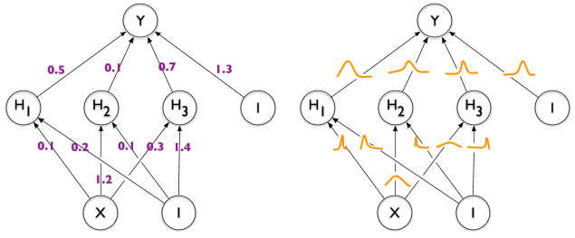
Graphical model under consideration. Solid lines denote the generative model $p_{\theta}(z) p_{\theta}(x|z)$ while dashed lines denote the variational approximation $q_{\phi}(z|x)$ to the intractable posterior $p_{\theta}(z|x) $ From [1]'s slides

The variational bound:
$\log p_{\theta}(x^{(1)}, ..., x^{(N)})=\sum_{i=1}^N \log p_{\theta} (x^{(i)})$
for each $i$:
\begin{align}
\log p_{\theta}(x^{(i)})&=E_{z \sim q_{\phi}(z|x^{(i)}) } [\log p_{\theta}(x^{(i)})] \\

&=E_z [\log \frac{p_{\theta}(x^{(i)} |z) p_{\theta}(z)} {p_{\theta}(z | x^{(i)} ) }]  \: (\textrm{Bayes' Rule}) \\

&=E_z[\log \frac{p_{\theta}(x^{(i)} |z) p_{\theta}(z)} {p_{\theta}(z | x^{(i)} ) }  \frac{ q_{\phi} (z| x^{(i)}) } {q_{\phi} (z| x^{(i)}) } ] \\

&=E_z [ \log p_{\theta} ( x^{(i)} | z)] - E_z[ \log \frac{q_{\phi} (z| x^{(i)}) }{p_{\theta}(z) }] + E_z [ \log \frac{q_{\phi} (z| x^{(i)}) } {p_{\theta}(z | x^{(i)}) }] \\
&=\color{red} { E_z[ \log p_{\theta} ( x^{(i)} | z)] } - \color{green}{  D_{KL}( q_{\phi} (z| x^{(i)}) || p_{\theta}(z) ) } +\color{blue} { D_{KL}( q_{\phi} (z| x^{(i)}) || p_{\theta}(z | x^{(i)})) }\\

&= \mathcal{L}(\theta, \phi; x^{(i)}) +  D_{KL}( q_{\phi} (z| x^{(i)}) || p_{\theta}(z | x^{(i)})) \\

&\ge  \mathcal{L}(\theta, \phi; x^{(i)}) \: \textrm{(Variational lower bound)}
\end{align}

In the red term, $ \log p_{\theta} ( x^{(i)} | z)]$ is the probability of $x^{(i)}$ given $z$ we have sampled. This term is greater if given true ( or more "truthful") latent encoding $z|x^{(i)}$. Therefore, red term is also called reconstruction error/loss.

Green term is the KL between probabilistic encoder $q_{\phi} (z| x^{(i)})$ and prior $p_{\theta}(z)$. It encourages the model to learn some more interesting latent encoding rather than simply encoding an identity mapping. This term is called regularization term.

Blue term is the KL between two intractable posteriors. To my knowledge there isn't good way to deal with it. We simply acknowledge this is a non-negative term.

Red term minus green term yields the classical variational lower bound:
\begin{align}
\mathcal{L}(\theta, \phi; x^{(i)}) &= E_z[ \log p_{\theta} ( x^{(i)} | z)]  -  D_{KL}( q_{\phi} (z| x^{(i)}) || p_{\theta}(z) ) \\

&=E_z[ \log p_{\theta} ( x^{(i)} ,z) - \log q_{\phi} (z| x^{(i)}) ]
\end{align}

Possible ways to deal with this bound:
Define：
$f_{\theta, \phi}(z)= \log p_{\theta} ( x^{(i)} ,z) - \log q_{\phi} (z| x^{(i)})  $
$$
\begin{align}
\mathcal{L}(\theta, \phi; x^{(i)}) &= E_{q_{\phi}(z|x^{(i)})}[f_{\theta, \phi}(z)] \\
&\approx \frac{1}{L} \sum_{i=1}^L f_{\theta, \phi}(z^{(l)}) \:\textrm{(Monte Carlo Estimator of this bound)}
\end{align}
$$

where $z^{(l)} \sim q_{\phi}(z|x)$


We also need to compute the gradient:
$ \nabla_{\theta, \phi} E_{q_\phi(z)} \left [ \log p_\theta(x,z) - \log q_\phi(z|x) \right] $



For $\nabla_{\theta}$ things are not too hard:
$ \nabla_{\theta} E_{q_\phi(z)} \left [ f_{\theta, \phi}(z) \right]=E_{q_\phi(z)} \left[ \nabla_{\theta} \log p_\theta(x,z) \right]
 $

For $\nabla_{\phi}$ things become a bit more complicated:
\begin{align}
\nabla_{\phi} E_{q_\phi(z)} \left [ f_{\theta, \phi}(z) \right] &= \nabla_{\phi} E_{q_\phi(z)} \left [ \log p_\theta(x,z) - \log q_\phi(z|x) \right] \\

&= \nabla_{\phi} \int{\log p_\theta(x,z)  q_\phi(z|x) dz} -\nabla_{\phi} \int{q_\phi(z|x) \log q_\phi(z|x) dz }\: \textrm{(Assuming continuous  latent variable case)} \\

&=\int{\log p_\theta(x,z) \nabla_{\phi} q_\phi(z|x) dz} - \int{(\log q_\phi(z|x) +1) \nabla_{\phi}
q_\phi(z|x)  dz } \\
&= \int{ (\log p_\theta(x,z) - \log q_\phi(z|x) )  \nabla_{\phi}  q_\phi(z|x)  dz }
\end{align}

where we use the fact that
 $$
\begin{align}
\int{ \nabla_{\phi}  q_\phi(z|x)  dz  } &=\nabla_{\phi}\int{   q_\phi(z|x)  dz  } \\
&=  \nabla_{\phi} 1 \\
&= 0
\end{align}
$$

Again, we use the identity
$\nabla_{\phi}  q_\phi(z|x) =  q_\phi(z|x)  \nabla_{\phi} \log{q_\phi(z|x) }$
(Why? Because $\nabla_{\phi} \log{q_\phi(z|x) }= \frac{ \nabla_{\phi} q_\phi(z|x) } {q_\phi(z|x) }q_\phi(z|x) $) )

So we have:
\begin{align}
\nabla_{\phi} E_{q_\phi(z)} \left [ f_{\theta, \phi}(z) \right] &= \nabla_{\phi} E_{q_\phi(z)} \left [ \log p_\theta(x,z) - \log q_\phi(z|x) \right] \\

&=\int{ (\log p_\theta(x,z) - \log q_\phi(z|x) )  \nabla_{\phi}  q_\phi(z|x)  dz } \\

&=\int{ (\log p_\theta(x,z) - \log q_\phi(z|x) )  q_\phi(z|x)  \nabla_{\phi} \log{q_\phi(z|x) } }\\

&=\color{red } { E_{q_\phi(z|x)} [ (\log p_\theta(x,z) - \log q_\phi(z|x) )   \nabla_{\phi}\log{q_\phi(z|x) }   ] }

\end{align}

An possible estimator can be:
\begin{align}
\nabla_{\phi} E_{q_\phi(z)} \left [ f_{\theta, \phi}(z) \right]
&=\color{red } { E_{q_\phi(z|x)} [ (\log p_\theta(x,z) - \log q_\phi(z|x) )   \nabla_{\phi}\log{q_\phi(z|x) }   ] } \\

&\approx \color{blue}{\frac{1}{L} \sum_{l=1}^L f_{\theta, \phi}(z) \nabla_{\phi}   \log q_\phi(z^{(i)} |x)}

\end{align}

where $z^{(l)} \sim q_{\phi}(z|x)$
However, this estimator exhibits very high variance.

Re-parameterization trick:
The core of re-parameterization trick is to rewrite the $q_{\phi}(z|x)$ in terms of a deterministic mapping $g$ of both $x$ and auxiliary noise variable $\epsilon $ sampled from some probability distribution $p(\epsilon)$.
i.e.:
$\widetilde{\mathbf{z}}=g_{\phi}(\epsilon, \mathbf{x})$ with $\boldsymbol{\epsilon} \sim p(\boldsymbol{\epsilon})$

Re-parameterization moves the random part to the $\epsilon$ which is reflected in the sampling process. Picture from [1].

Now the Monte Carlo estimates of the expectations of  some function $f(z)$ w.r.t. $q_{\phi}(z|x)$ is as follows:
$\mathbb{E}_{q_{\phi}\left(\mathbf{z} | \mathbf{x}^{(i)}\right)}[f(\mathbf{z})]=\mathbb{E}_{p(\epsilon)}\left[f\left(g_{\phi}\left(\boldsymbol{\epsilon}, \mathbf{x}^{(i)}\right)\right)\right] \simeq \frac{1}{L} \sum_{l=1}^{L} f\left(g_{\phi}\left(\boldsymbol{\epsilon}^{(l)}, \mathbf{x}^{(i)}\right)\right)$

where
$\boldsymbol{\epsilon}^{(l)} \sim p(\boldsymbol{\epsilon})$.

And the variational lower bound can be approximated rewritten in two ways, yielding two Stochastic Gradient Variational Bayes Estimator :
$$\begin{align} \mathcal{L}\left(\boldsymbol{\theta}, \boldsymbol{\phi} ; \mathbf{x}^{(i)}\right) &\approx \widetilde{\mathcal{L}}^{A}\left(\boldsymbol{\theta}, \boldsymbol{\phi} ; \mathbf{x}^{(i)}\right) \\

&=\color{blue} { \frac{1}{L} \sum_{l=1}^{L} \log p_{\boldsymbol{\theta}}\left(\mathbf{x}^{(i)}, \mathbf{z}^{(i, l)}\right)-\log q_{\boldsymbol{\phi}}\left(\mathbf{z}^{(i, l)} | \mathbf{x}^{(i)}\right) }
 \end{align} $$

where $\mathbf{z}^{(i, l)}=g_{\phi}\left(\boldsymbol{\epsilon}^{(i, l)}, \mathbf{x}^{(i)}\right)$
and $\boldsymbol{\epsilon}^{(l)} \sim p(\boldsymbol{\epsilon})$

2. Often the KL-divergence $D_{K L}\left(q_{\phi}\left(\mathbf{z} | \mathbf{x}^{(i)}\right) \| p_{\boldsymbol{\theta}}(\mathbf{z})\right)$ can be integrated analytically (especially true when both distributions are gaussians) leading to our second version of estimator:

$$\begin{align} \mathcal{L}\left(\boldsymbol{\theta}, \boldsymbol{\phi} ; \mathbf{x}^{(i)}\right) &\approx \widetilde{\mathcal{L}}^{B}\left(\boldsymbol{\theta}, \boldsymbol{\phi} ; \mathbf{x}^{(i)}\right) \\

&=\color{blue} {-D_{K L}\left(q_{\phi}\left(\mathbf{z} | \mathbf{x}^{(i)}\right) \| p_{\boldsymbol{\theta}}(\mathbf{z})\right)+\frac{1}{L} \sum_{l=1}^{L}\left(\log p_{\boldsymbol{\theta}}\left(\mathbf{x}^{(i)} | \mathbf{z}^{(i, l)}\right)\right)}
 \end{align} $$
where $\mathbf{z}^{(i, l)}=g_{\phi}\left(\boldsymbol{\epsilon}^{(i, l)}, \mathbf{x}^{(i)}\right)$
and $\boldsymbol{\epsilon}^{(l)} \sim p(\boldsymbol{\epsilon})$

When given multiple datapoints from dataset $X={x^{(i)} }_{i=1}^N $, we can construct an estimator based on mini-batches:
$\mathcal{L}(\boldsymbol{\theta}, \boldsymbol{\phi} ; \mathbf{X}) \simeq \widetilde{\mathcal{L}}^{M}\left(\boldsymbol{\theta}, \boldsymbol{\phi} ; \mathbf{X}^{M}\right)=\frac{N}{M} \sum_{i=1}^{M} \widetilde{\mathcal{L}}\left(\boldsymbol{\theta}, \boldsymbol{\phi} ; \mathbf{x}^{(i)}\right)$

where $\mathbf{X}^{M}=\left\{\mathbf{x}^{(i)}\right\}_{i=1}^{M}$ is the randomly drawn sample.

$\nabla_{\boldsymbol{\theta}, \boldsymbol{\phi}} \widetilde{\mathcal{L}}\left(\boldsymbol{\theta} ; \mathbf{X}^{M}\right)$ can be taken, of course.

The intuition behind this re-parameterization trick is:
we want to find to find some $p(\epsilon)$ such that
$q_{\phi}(\mathbf{z} | \mathbf{x}) \prod_{i} d z_{i}=p(\epsilon) \prod_{i} d \epsilon_{i}$
therefore, $\int q_{\phi}(\mathbf{z} | \mathbf{x}) f(\mathbf{z}) d \mathbf{z}=\int p(\boldsymbol{\epsilon}) f(\mathbf{z}) d \boldsymbol{\epsilon}=\int p(\boldsymbol{\epsilon}) f\left(g_{\phi}(\boldsymbol{\epsilon}, \mathbf{x})\right) d \boldsymbol{\epsilon}$
and so a differentiable estimator can be constructed: $\int q_{\phi}(\mathbf{z} | \mathbf{x}) f(\mathbf{z}) d \mathbf{z} \simeq \frac{1}{L} \sum_{l=1}^{L} f\left(g_{\phi}\left(\mathbf{x}, \epsilon^{(l)}\right)\right)$ where $\boldsymbol{\epsilon}^{(l)} \sim p(\boldsymbol{\epsilon})$.

Concrete ways of finding reparameterizations can be found from the original paper[7].

But the author didn't mention why re-parameterization helps alleviate variance, possible explanations can be found in the appendix section of [8].

Ref:

1. Kingma's NIPS 2015 workshop slides
2. Kingma's Stochastic Gradient VB. Intractable posterior distributions? Gradients to the rescue!
3. https://ermongroup.github.io/cs228-notes/extras/vae/
4. CS231n Lecture 11 Slides 
5. Mnih, A., & Gregor, K. (n.d.). Neural Variational Inference and Learning in Belief Networks. 
6. Openreview page for the original paper
7. Kingma, D., & Welling, M. (2014). Auto-Encoding Variational Bayes
8. Rezende, D., Mohamed, S., & Wierstra, D. (2014). Stochastic Backpropagation and Approximate Inference in Deep Generative Models. 

What is reinforcement learning?

A lot of people might think this question is obvious. It's just a bunch of methods for optimizing behavior for an agent in some environment based on reward signals.

• But what's its history? 
• How does it relate to optimization problem or traditional optimal control problem? 
• How is it different from supervised or unsupervised learning?
•  Why it's named "reinforcement learning" instead of "optimal behavior learning". 
• Does the "reinforcement" word suggest something special?

Can you answer these questions?

Approximate dynam-ic programming (ADP) has emerged as a powerful tool for tackling a diverse collection of stochastic optimization problems. Reflecting the wide diversity of problems, ADP (including research under names such as reinforcement learning, adaptive dynamic programming and neuro-dynamic programming) has become an umbrella for a wide range of algorithmic strategies. Most of these involve learning functions of some form using Monte Carlo sampling. A recurring theme in these algorithms involves the need to not just learn policies, but to learn them quickly and effectively. Learning arises in both offline settings (training an algorithm within the computer) and online settings (where we have to learn as we go). Learning also arises in different ways within algorithms, including learning the parameters of a policy, learning a value function and learning how to expand the branches of a tree.

Approximate Dynamic Programming, First edition. By Frank Lewis and Derong Liu 

This book seems to view the so-called "reinforcement learning" as an alias for approximate dynamic programming which is used for solving stochastic optimization problems. So:

Reinforcement Learning= Approximate Dynamic Programming?

Also:

The term “ADP” can be interpreted either as “Adaptive Dynamic Programming” (with apologies to Warren Powell) or as “Approximate Dynamic Programming” (as in much of my own earlier work). The long-term goal is to build systems which include both capabilities; therefore, I will simply use the acronym “ADP” itself. Various strands of the field have sometimes been called “reinforcement learning” or “adaptive critics” or “neurodynamic programming,” but the term “reinforcement learning” has had many different meanings to many different people.

Learning And Approximate Dynamic Programming. By Jennie Si, Andy Barto, Warren Powell, and Donald Wunsch 

By the way, this book  or this paper  has drawn a comparison between supervised learning and reinforcement learning. Also you can find that comparison in Sutton and Barton's Reinforcement Learning book.  

Why is it called reinforcement learning?

The term reinforcement comes from studies of animal learning in experimental psychology, where it refers to the occurrence of an event, in the proper relation to aresponse, that tends to increase the probability that the response will occur againin the same situation. The simplest reinforcement learning algorithms make use ofthe commonsense idea that if an action is followed by a satisfactory state of affairs,or an improvement in the state of affairs, then the tendency to produce that actionis strengthened, i.e., reinforced. This is the principle articulated by Thorndike inhis famous “Law of Effect” (Thorndike, 1911). Instead of the term reinforcementlearning, however, psychologists use the terms instrumental conditioning, or operantconditioning, to refer to experimental situations in which what an animal actuallydoes is a critical factor in determining the occurrence of subsequent events. Thesesituations are said to include response contingencies, in contrast to Pavlovian, orclassical, conditioning situations in which the animal’s responses do not influencesubsequent events, at least not those controlled by the experimenter. There are verymany accounts of instrumental and classical conditioning in the literature, and thedetails of animal behavior in these experiments are surprisingly complex. See, forexample, Hergenhahn & Olson, 2001. The basic principles of learning via reinforcement have had an influence on engineering for many decades (e.g., Mendel &McClaren, 1970) and on Artificial Intelligence since its very earliest days (Minsky,1954, 1961; Samuel 1959; Turing, 1950). It was in these early studies of artificiallearning systems that the term reinforcement learning seems to have originated. Sut-vi REINFORCEMENT LEARNING AND ITS RELATIONSHIP TO SUPERVISED LEARNINGton and Barto (1998) provide an account of the history of reinforcement learning inArtificial Intelligence.But the connection between reinforcement learning as developed in engineeringand Artificial Intelligence and the actual details of animal learning behavior is farfrom straightforward. In prefacing an account of research attempting to capturemore of the details of animal behavior in a computational model, Dayan (2002)stated that “Reinforcement learning bears a tortuous relationship with historical andcontemporary ideas in classical and instrumental conditioning.” This is certainly true,as those interested in constructing artificial learning systems are motivated more bycomputational possibilies than by a desire to emulate the details of animal learning.This is evident in the view of reinforcement learning as a combination of search andlong-term memory discussed above, which is a an abstract computational view thatdoes not attempt to do justice to all the subleties of real animal learning.For our mobile phone example, the principle of learning by reinforcement isinvolved in several different ways depending on what grain size of behavior weconsider. We could think of a move in a particular direction as a unit of behavior,being reinforced when reception improved, in which case we would tend to continueto move in the same direction. Another view, one that includes long-term memory,is that the tendency to make a call from a particular place is reinforced when a callfrom that place is successful, thus leading us to increase the probability that we willmake a call from that place in the future. Here we see the reinforcement processmanifested as the storing in long-term memory of the results of a successful search.Note that the principle of learning via reinforcement does not imply that only gradualor incremental changes in behavior are produced. It is possible for complete learningto occur on a single trial, although gradual changes in behavior make more sensewhen the contingencies are stochastic.

Dietterich, A. G. B. T. G. (2004). Reinforcement learning and its relationship to supervised learning. Handbook of learning and approximate dynamic programming, IEEE, 47-60.

Neural Architecture Search

Max Welling's "Intelligence Per Kilowatt-Hour"

Complement of this blog post.

The talk starts from high-level physics analogy but in fact it's about energy-efficient machine learning in the end. In this blog post I am more interested in physics part.

Helmholtz: Free Energy=  Energy - Entropy 

What is the "ability to perform physical work"?

What is the "level of organization, information of  a system"? He didn't explain. 

It From Bit 

Entropic Forces and Gravity
Entropy is degree of ignorance
Bayes
Rissanen: Minimum Description Length Principle
Hinton: Variational Methods
Large Scale Approximate Bayesian Learning: MCMC versus Variational Bayes  

Those measurements for two probability distributions

f-divergence

Also known as Csiszár ƒ-divergences, Csiszár-Morimoto divergences or Ali-Silvey distances

Given two distributions $P$ and $Q$ which are both absolutely continuous w.r.t. a reference distribution $\mu$ on $\Omega$  and:

• $dP=pd\mu$
• $dQ=qd\mu$

$D_f(P||Q)=\int_\Omega f \frac{p(x)}{q(x)} q(x) d\mu(x)$

What is a cross-entropy loss function?

A lot of machine learning resources tend to be vague in giving definitions. This is because the authors don't know these concepts well enough.

So, what is a cross-entropy?

KL divergence(discrete form):
$KL(p||q)=\sum_{k=1}^K p_k log (\frac{p_k}{q_k})$
$KL(p||q)=\sum_k p_k log p_k -\sum_k p_k log q_k=-H(p)+ H(p,q)$

Here, $H(p)$ is the entropy for distribution $p$, $H(p,q)$ is the cross entropy between distribution $p$ and $q$, notice cross-entropy, like KL divergence, is asymmetric.

According to Cover and Thomas 2006, cross entropy is the average number of bits needed to encode data coming from a source with a distribution $p$ when we use model $q$ to define our cookbook.
Hence the "regular" entropy is $H(p)=H(p,p)$.

So what is a cross-entropy loss function, then?
Be patient, look at where does  a maximum log likelihood come from.

You may have seen the derivation of MLE (Maximum Likelihood Estimation) several times. You assume:

• Data is i.i.d distributed (recent years we have seen researches on non-i.i.d. data, but not for this article)
• $X={x^{(1)},..., x^{(m)}}$
• $p_{model}(x;\theta)$ is a parametric family of probability distributions over the data

$\theta_{ML}=argmax_{\theta} p_{model}(X; \theta)=argmax_{\theta} \sum_{i=1}^m p_{model}(x^{(i)}; \theta)$

It doesn't matter if you take the log likelihood because they are all positive:

$argmax_{\theta} \sum_{i=1}^m log( p_{model} (x^{(i)}; \theta))$

Divided  by $m$， it becomes:

$\theta_{ML}=argmax_{\theta} E_{x \sim  \tilde{p}_{data}} log p_{model} (x; \theta)$

Notice:

$KL(\tilde{p}_{data} || p_{model})=E_{x \sim  \tilde{p}_{data}} [log \tilde{p}_{data}(x) - log p_{model}(x) ]$

Minimizing over $KL(\tilde{p}_{data} || p_{model})$ w.r.t our model is equivalent to minimizing for the cross entropy term:

$-E_{x \sim  \tilde{p}_{data}} [log p_{model} (x)]=H(\tilde{p}_{data} || p_{model})$

This is also equivalent to MLE above. In fact, any loss consisting of a negative log-likelihood is a cross-entropy between the empirical distribution and probability distribution defined by the model.  e.g., mean squared error is the cross-entropy between the empirical distribution and a Gaussian model. The term "cross-entropy" used to refer negative log-likelihood (NLL) for a Bernoulli(logistic regression) or softmax distribution  is a misnomer because cross-entropy is in fact used in machine learning wherever there is a maximum likelihood.
--------------------------------
2019.5.18 Note:
For many discriminative models, the above formulas aren't very accurate. Concretely:

• $X=\{x^{(i)}\}_{i=1}^n \times Y=\{y^{(i)}\}_{i=1}^n \sim \tilde{p}_{data}$

• $$\theta_{ML}=argmax_{\theta} p_{model}(Y|X, \theta)=argmax_{\theta} \sum_{i=1}^m p_{model}(y^{(i)} | x^{(i)}, \theta)$$
• $\theta_{ML}=argmax_{\theta} E_{x,y \sim  \tilde{p}_{data}}[ log p_{model} (y | x, \theta)]$
• Then it can seen as minimize cross-entropy: $-E_{x,y \sim  \tilde{p}_{data}}[ log p_{model} (y | x, \theta)]=H(\tilde{p}_{data}(y|x) || p_{model}(y|x, \theta))$
• Or you can see it from KL divergence perspective: $argmin_{\theta} KL(\tilde{p}_{data}(y|x) || p_{model}(y|x))=argmin_{\theta} E_{x,y \sim  \tilde{p}_{data}} [log \tilde{p}_{data}(y|x) - log p_{model}(y|x) ]=argmin_{\theta} H(\tilde{p}_{data}(y|x) || p_{model}(y|x, \theta))$

Reference:

1. Goodfellow, I., Bengio, Y., & Courville, A. (2016). Deep learning. MIT press.
   
2. Murphy, K. P. (2012). Machine learning: a probabilistic perspective. MIT press.
   

Doing Things in a Reverse Way---those reverse operations in machine learning

Deconvolution

Geometric Deep Learning?

I found a new website: http://geometricdeeplearning.com/
Good tutorials:

• Joan Bruna NIPS 2017 Geometric Deep Learning on Graphs and Manifolds
• PDF tutorial:https://arxiv.org/pdf/1611.08402.pdf
• Xavier Bresson: "Convolutional Neural Networks on Graphs"
• Slides: http://helper.ipam.ucla.edu/publications/dlt2018/dlt2018_14506.pdf

Basically in the tutorial Joan introduced the concept of manifold and graph theories. And then derived spectral graph convolution operations. What is missing is how can CNN be applied to general manifold instead of Euclidean space and graph? 

All because of computational power

Convolution(1)

• How to compute the size of the Conv layer?

Supoose:

1. S:= # Stride 
2. N := output size
3. F:= Filter size
4. P:=Padding size

Think about all these heads

$W+2P=(F-1)+(N-1)*S+1$

which gives 

$N=\frac{W+2P-F}{S}+1$

Famous CS231n only gives you the formula but does not tell you why. 

Why real symmetric matrices are diagonalizable with real eigenvalues?

Graph Convolution Neural Nets? Are you out of your mind? How can you do this on a graph?

Recently I am working on reproducing the paper Graph Convolutional Matrix Completion . A natural question to ask is what is convolution on graph.

Convolution at first is defined for continuous space, later maybe signal processing guy has extended this idea to discrete space(say image processing, the convolutional kernel you used in convolutional neural network). But what about graphs?

The first idea may appeared in Joan Bruna's this paper. Then extended by Defferrard et al(2016).
The version I encountered is Thomas N. Kipf et al.(2017), which I will introduce here.

The basic setting is here:

• $x\in R^N$ is a feature vector of the nodes of a graph 
• Convolutional kernel/filter $g_\theta=diag(\theta), \theta\in R^N$ lies in the Fourier domain

$g_\theta * x = Ug_\theta U^T x$
where $U$ is the matrix of eigenvectors of the normalized graph Laplacian $L=I_N-D^{-1/2}AD^{-1/2}=U \Lambda U^T$ , where $D_{i, i}=\sum_j {A_{i, j }}$

Note:

1. In spectral-based models, graph are assumed to be undirected. Normalized graph Laplacian matrix is one representation.  
2. Graph Fourier Transform: $\mathcal{F}(x)= U^T x$
3. Inverse Graph Fourier Transform: $\mathcal{F}^{-1}(\hat{x})= U \hat{x}$
4. Derivation: 

\begin{align}
g_\theta * x & = \mathcal{F}^{-1} (\mathcal{F}(x)  \odot \mathcal{F}(g)) \\
& = Ug_\theta U^T x
\end{align}

They are not satisfied, yet. Computing $g_\theta$ is expensive, so they use an approximation derived in Hammond et al.(2011), where:
$g_\theta'(\Lambda) \approx \sum_{k=0}^K \theta_k^{'}T_k(\tilde{\Lambda})$
where $T_k(x)$ is the Chebyshev polynomials. $T_0(x)=1, T_1(x)=x, T_k(x)=2xT_{k-1}(x)-T_{k-2}(x) $
$\tilde{\Lambda}=\frac{2}{\lambda_{max}} \Lambda - I_N$, $\lambda_{max}$ is the largest eigenvalue of $L$

They limit the $K=1$, and assume $\lambda_{max}\approx2$

Now:
$g_{\theta'}*x\approx \theta_0'x+\theta_1^{'}(L-I_N)x=\theta_0^{'}x-\theta_1^{'}D^{-\frac{1}{2}}AD^{-\frac{1}{2}}x$

Further, they assume $\theta=\theta_0^{'}=-\theta_1^{'}$

Apply re-normalization trick to prevent exploding/vanishing gradients problem:

1. $\tilde{A}=A+I_N$
2. $\tilde{D}_{ii}=\sum_j \tilde{A}_{ij}$
3. $I_N+D^{-\frac{1}{2}}AD^{-\frac{1}{2}} \rightarrow \tilde{D}^{-\frac{1}{2}} \tilde{A} \tilde{D}^{-\frac{1}{2}}$

Matrix representation:

Suppose $X\in R^{N \times C} $  is the signal/input, where C is the dim of input channels/features. $\Theta\in R^{C \times F }$ a matrix of filter parameters. $Z \in R^{N \times F}$ is the convolved 

input matrix.

$Z=\tilde{D}^{-\frac{1}{2}} \tilde{A} \tilde{D}^{-\frac{1}{2}} X \Theta $

Ref:

1.

Mathjax test

Spanning multiple lines(Aligned equations):
\begin{align}
\sqrt{37} & = \sqrt{\frac{73^2-1}{12^2}} \\
 & = \sqrt{\frac{73^2}{12^2}\cdot\frac{73^2-1}{73^2}} \\
 & = \sqrt{\frac{73^2}{12^2}}\sqrt{\frac{73^2-1}{73^2}} \\
 & = \frac{73}{12}\sqrt{1 - \frac{1}{73^2}} \\
 & \approx \frac{73}{12}\left(1 - \frac{1}{2\cdot73^2}\right)

\end{align}